Tutorial 2: Steady-state hyper-elasticity

Objective: At the end of this tutorial you will understand how to use this software framework to solve the steady-state solid mechanics problem.

We consider a large deformation hyper-elastic non-linear material model applied to a cubical box. The strong form of this problem can be expressed as follows: find the displacement \(\mathbf{U} : \Omega \rightarrow \mathbb{R}^3\) such that

(1)\[\begin{split}\begin{align} \nabla \cdot \mathbf{P} &= 0 \quad \text{in} \ \Omega, \\ \mathbf{U} &= \mathbf{g} \quad \text{on} \ \Gamma_D, \\ \mathbf{P} \cdot \mathbf{n} &= 0 \quad \text{on} \ \Gamma_N, \end{align}\end{split}\]

where \(\mathbf{P}\) is the first Piola-Kirchhoff stress tensor, \(\mathbf{g}\) is the prescribed displacement on the Dirichlet boundary \(\Gamma_D\), \(\mathbf{n}\) is the outward normal of the Neumann boundary \(\Gamma_N\) defined in the reference configuration of the domain. In our material model, the second Piola-Kirchhoff stress tensor \(\mathbf{S}\) is related to the right Cauchy-Green strain tensor \(\mathbf{C}\) by the relationship

\[\mathbf{S} = \mu \left( \mathbf{I} - \mathbf{C}^{-1} \right) + \frac{\lambda}{2} \left(J^{2} - 1 \right) \mathbf{C}^{-1},\]

where \(\mathbf{C} = \mathbf{F}^T \mathbf{F}\) is the right Cauchy-Green deformation tensor, \(\mathbf{F}\) is the deformation gradient, \(J = \det(\mathbf{F})\), and \(\lambda, \mu\) are the Lamé constants from linear elasticity. The first Piola-Kirchhoff stress tensor is defined by \(\mathbf{P} = \mathbf{F} \mathbf{S}\) and the symmetry condition \(\mathbf{P}^T \mathbf{F} = \mathbf{F}^T \mathbf{P}\) holds.

We solve the linearized weak form of the equations given by (1) in an updated-Lagrangian approach; see the code-snippet below (in src/hyperelastic/HyperElasticity.c) for its implementation.

PetscInt step;
for(step=0;step<nsteps;step++)
{
   PetscPrintf(PETSC_COMM_WORLD,"%d Load Step\n",step);

   // Solve step
   ierr = VecZeroEntries(U);CHKERRQ(ierr);
   ierr = SNESSolve(snes,NULL,U);CHKERRQ(ierr);

   // Store total displacement
   ierr = VecAXPY(Utotal,1.0,U);CHKERRQ(ierr);

   // Update the geometry
   if(iga->geometry)
   {
      Vec localU;
      const PetscScalar *arrayU;
      ierr = IGAGetLocalVecArray(iga,U,&localU,&arrayU);CHKERRQ(ierr);
      PetscInt i,N;
      ierr = VecGetSize(localU,&N);
      for(i=0;i<N;i++) iga->geometryX[i] += arrayU[i];
      ierr = IGARestoreLocalVecArray(iga,U,&localU,&arrayU);CHKERRQ(ierr);
   }

   // Dump solution vector
   char filename[256];
   sprintf(filename,"disp%d.dat",step);
   ierr = IGAWriteVec(iga,Utotal,filename);CHKERRQ(ierr);
}

We consider the domain to be a rectangular box discretized with a mesh of 32 x 32 x 32 quadratic B-spline functions. The right side of the box is fixed and the left side is displaced to the left over 15 load steps. We run the code src/hyperelastic/HyperElasticity.c by passing the parameters in src/hyperelastic/params.txt to the executable as follows: mpirun ./Hyperelasticity -options_file params.txt > output.o. The output of the code is the displacement field of the box in the deformed configuration (see below), which can be visualized via the python script src/hyperelastic/postp.py that uses the IGAKIT library.

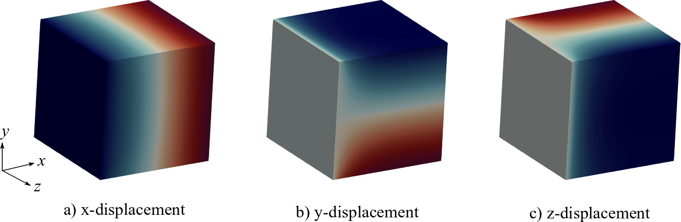
Figure: Displacements in the deformed box.

For the numerical solution, we use Newton-Raphson method with a backtracking line-search as the non-linear solver; see src/hyperelastic/params.txt for more details.