Tutorial 3: unsteady incompressible Navier-Stokes equations
Objective: At the end of this tutorial you will understand how to use this software framework to solve the unsteady fluid mechanics problem.
We solve the incompressible Navier-Stokes equations stabilized with the variational multiscale method as formulated in [1]. Let \(\Omega \subset \mathbb{R}^d\) be an open set, where \(d=2,3\). The boundary of \(\Omega\) with unit outward normal is denoted \(\Gamma\). The problem can be stated in strong form as: find the dimensionless fluid velocity \(\mathbf{u}: \Omega \times (0,T) \rightarrow \mathbb{R}^d\) and the dimensionless pressure \(p: \Omega \times (0,T) \rightarrow \mathbb{R}\) such that,
where \(\mathbf{u}_0\) is the initial velocity, \(\mathbf{f}\) represents the dimensionless body force per unit volume, and \(\nu\) is the dimensionless kinematic viscosity (also equal to the Reynolds number). We solve a turbulent flow in a rectangular box the results of which we plot in Figure: Turbulent flow in a rectangular box. The plot shows the iso-contours of the Q-criterion..
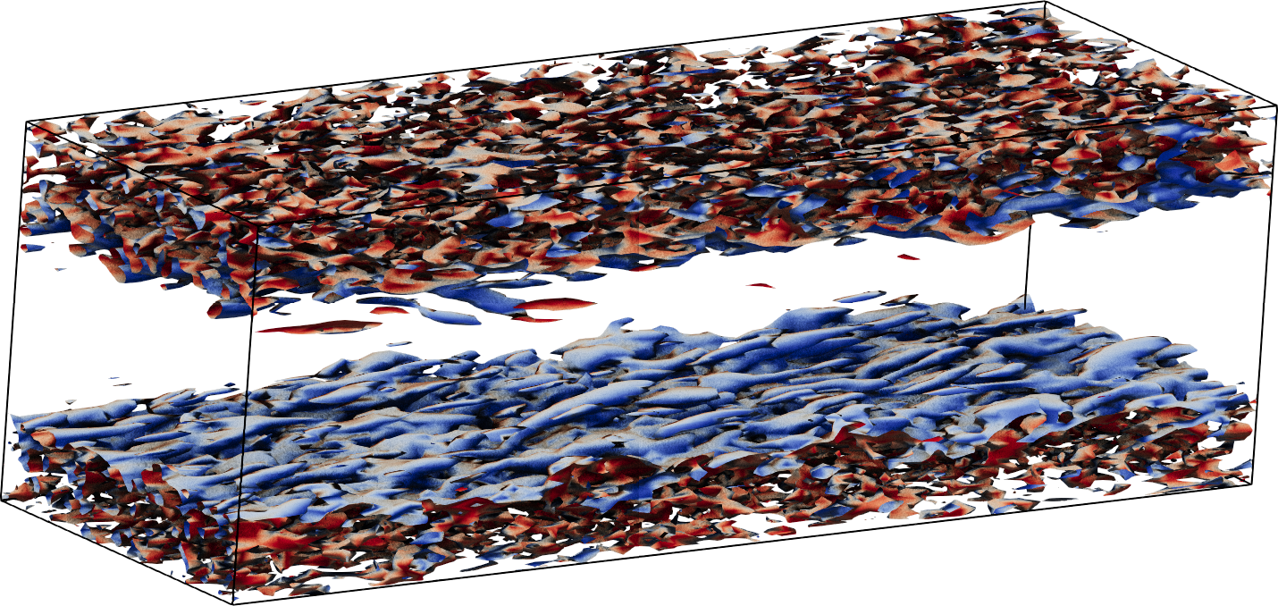
Figure: Turbulent flow in a rectangular box. The plot shows the iso-contours of the Q-criterion.
For the simulations, we assume that the domain is periodic in the streamwise direction, which we set using the function IGAAxisSetPeriodic in the code src/nse/NavierStokesVMS.c. We set no-slip boundary conditions at the top and bottom boundaries and we set the initial condition using a laminar flow profile. The simulation is forced using a pressure gradient in the form of a body force in the streamwise direction. We run the code src/nse/NavierStokesVMS.c by passing the parameters in src/nse/params.txt to the executable as follows: mpirun ./NavierStokesVMS -options_file params.txt > output.o. The output of the code are the fluid variables (\(\mathbf{u}\) and \(p\)) in the box, which can be visualized via the python script src/nse/postp.py that uses the IGAKIT library.